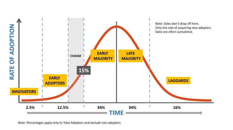
Technology Adoption Curve Examples – The life cycle depends on technology technology (TALC) is a graphic fee that every innovative investor must be wrong with it. Talc notes that the time adopted by different people follow a new technology that follows the distribution of the bell curve. Initially, a few enthusiasts and technology visions depend. It is adopted by the vast majority at some point in the middle, and the few skeptics are not satisfied near the end of the life cycle.
However, the number of new adopters is not related to the total consumer in anticipation of product sales. Consumers can be divided into customers for the first time to buy the first and current customers who replace the products. As we reach the vast majority of talc, the first time customers begin to bypass the market, which quickly increases the total sales. As we enter the late majority, there is a flow point when selling a product where the rate of new customers begins to slow down, which also slows down the rate of sales increase. In the end, all sales come from the replacement of the product, but since many customers who have adopted technology now, sales are still higher than the highest level at all times.
Technology Adoption Curve Examples

Since Talc creates the S curve, we can use the SC Universal curve equation for the growth model. If you are interested in how to reap this equation, I will explain in more detail here.
The State Of Enterprise Ai Adoption In 2024
Note that Tam, K and B are consistent, not variables, which means that they do not change over time. TAM can be easily estimated, but K and B are arbitrary that we will need to be resolved. How to do this is somewhat simple and will be explained in the next section.
We will now use the above equation for the EDD curve model. To do this, we will need two assumptions.
Annual global auto sales about 80 million. However, due to its less parts, EV is more reliable than the gas car, which reduces the number of sales of the replay of the product. However, after the world’s growing population, I think it is fair to preserve TAM at 80 million. Another implicit assumption is that EVS will represent 100 % of car sales sooner or later. Looking at the fact that it will be cheaper soon than the presence of gas, getting better, and more sustainable, I will follow this assumption.
This is more difficult. The choice of time is very early, such as 2005, will exaggerate the growth speed. On the other hand, choosing time is too late, such as 2020, will be reduced. We’ll play with this variable later, but let’s choose in 2015 as the start of the S-Curve at the present time.
Emerging Technologies: Trends, Challenges And Opportunities
Let’s now put our algebra hats and start providing a specific equation by finding Tam, B and K. Tam values equal to 80,000, 000 due to the first assumption. Moreover, since 540, additional car was sold in 2015, and we assume that 2015 is the beginning of the S curve, we know that R (0) = 540, 000.
Another part of our information is that 3.24 million additional components have been sold in 2020. Since 2020 after 5 years of 2015, we know R (5) = 3, 240, 000. Using this value and value B that we found, we can solve it for the lost final fixed, K.
Now, let’s rewrite the final equation using the B and K values that we discovered and we saw how it looks at her foolishness!

Figure 3: A model curve for annual EV sales growth. The X -years axis represents the number of years after 2015. The Y is the number of cars sold that year. The graph was found by drawing the above -equivalent graphs in Desmus.
Blockchain And Its Impact On Business Success
Figure 3 is the graph of the above equation. Note how the graphic cut is 540,000, which is the number of additional components sold in 2015. Point (5, 3 240,000) is also on the graph that represents 3.24 million vehicles sold per year 5 (2020). Moreover, we can expect this year’s EV World sales about 4.58 million. In fact, Since Since we started in 2015, the Since we started in 2015, the year will be 25 2040.
As you promised, we will now control the year in which the S. The following table shows the future sales prospects and the year in which the S-upling is settled. Accounts were made in the same way as mentioned previously. Unfortunately, 2010 is the first year in which we can get accurate data for the number of EVS that was sold that year, so no S -kinship s was designed at the beginning of a year before 2010.
The purpose of job modeling with different years is not to produce different sales expectations for 2021. Instead, it is supposed to highlight how changes in the beginning year affecting the largely used results.
Remember that the start year represents the beginning of the S. for EVS, the S curve did not start in 2018, and it did not start in 2015 or 2012 in this regard. The fine year is controversial, but in 2010 we are the closest to the beginning of the S -EVS curve. This means that if we want an accurate projection of future sales, we must use 2010 as a starting point.
Technology Adoption Curve: 5 Stages Of Adoption
Using points P (0) = 24, 500 and P (10) = 3, 240, 000 (where T is the number of years after 2010, so T = 10 means 2020) to solve the constants B and K as shown previously, we get the following equation.
To anticipate sales for 2021, let T = 11 expression rating. You must have a number of about 5, 192, 000. Note, as statistics use measured ingredients, which include hybrid. The pure EVS number is likely to be lower than this. You can also draw this yourself using the graph technology to find out the shape of the S curve and expects EV sales per year. Remember that T is equal to the number of years after 2010.
Possible delivery restrictions, demand restrictions, Wright law cannot be calculated, or how robotics can affect sales can be reasons for the belief that this model is wrong. However, in order to calculate the above -mentioned factors, you must put more assumptions. When you assume, the risk of your model will be incorrect. The only assumptions that this model has set are the total reference market and when the S. Each of these assumptions can be made with some certainty. This does not mean that this model is more accurate than all others, only that it should not be reduced due to its simplicity.

This is because there are more factors that affect the sale of a specific company of factors that affect the total industry. Many destroyed creators will be restricted at some point, which means that the company cannot produce enough products to meet all demand. This would cause sales to deviate from the standard S. Moreover, unexpected competitors can extract the market share from the current companies (imagine the use of Curve S for the Nokia growth model in 2007).
A Cognitive Model For Technology Adoption
3. On the theme of electric cars, this model can be used to predict the direction of Gigafactories over time
Since projects such as a newly built factory production curve is often the model used in this article can predict the number of cars that are produced monthly over a month. You don’t have to assume even when the S curve starts because it starts as soon as the factory starts production. In terms of the total reference market, this becomes its productive capacity as soon as the factory reaches the full capacity.
I want to conclude by comparing this model with ARK investment expectations regarding the EV market. ARK believes that technological progress will reduce the costs of the Wright Law and reduce the price/fees/fees. These positive contraction forces reduce prices and increase demand. In January 2020, Ark Investt expected 37 million in EV World sales in 2024. My model is more conservative, with sales of 37 million in 2025. I don’t know how accurate my model is, but I know it is completely fake.
From electric cars to the extermination of the genome, from Fintech to 3D printing, and from Blockchain to exploring the space, there is an innovation on the doorstep. While the irreversible Si growth of linear growth early, you know that the rate of adoption of new technologies will follow the frequent S curve. Also, you know that despite the shortcomings, the simple equation presented here will allow you to model the growth of emerging industries more accurately than many traditional analysts. It is difficult to adopt the product. People do not like change, and even when the benefits of adopting new technology are clear, there is always a lot of resistance.
On Things #1
Enter the adoption curve, known as the spread of innovations. This is a model for technology adoption